Exponential growth and decay: modelling with eˣ and ln x – Logarithmic and Exponential Functions (Senior 6 Mathematics) | Ganzaa

Logarithmic and Exponential Functions

Lessons

Senior 6 · Mathematics

Logarithmic and Exponential Functions

4 lessons

Lesson 4 of 4

Exponential growth and decay: modelling with eˣ and ln x

25 min

Rwanda's population, 2012 to 2022

The National Institute of Statistics of Rwanda (NISR) counted 10 515 973 people in the 2012 census and 13 246 394 in the 2022 census, an average growth of 2.3% a year (NISR, Fifth Population and Housing Census, Main Indicators, 2022). A population that grows by a steady percentage does not grow by the same number each year: the more people there are, the more children are born. Growth like this, where the rate of change is proportional to the amount present, is modelled by the exponential function. This lesson uses the calculus of Lessons 1 to 3 to build such models, find their parameters from real data, and judge how far to trust them. In S5 you solved exponential equations for similar problems; here you also differentiate the models and test them against data.

Definition

Exponential model: a quantity $y (t)$ whose rate of change is proportional to its size,

\frac{dy}{dt} = ky \quad (k \text{ constant}), \qquad \text{which gives} \qquad y = y_0 e^{kt},

where $y_{0} = y (0)$ is the initial amount. It is exponential growth if $k \gt 0$ and exponential decay if $k \lt 0$ . The constant $k$ is the continuous growth rate.

Why every solution has this form: if $y^{'} = k y$ , then $\frac{d}{dt}\left(ye^{-kt}\right) = y'e^{-kt} - kye^{-kt} = 0$ , so $ye^{-kt}$ is a constant, $y_{0}$ . Conversely, $\frac{d}{dt}\left(y_0 e^{kt}\right) = ky_0 e^{kt}$ . (Unit 5, Differential Equations, studies such equations in general.)

Important

Doubling time and half-life. For growth, $y = 2 y_{0}$ when $e^{kT} = 2$ , so the doubling time is $T = \frac{\ln 2}{k}$ . For decay ( $k \lt 0$ ), $y = \frac{1}{2}y_0$ when $e^{kT} = \frac{1}{2}$ , so the half-life is $T = \frac{\ln 2}{|k|}$ . Neither depends on $y_{0}$ : the time to double is the same whatever the starting amount.

Continuous and yearly rates: growth of $r$ per year (compounded yearly) is $y_0(1 + r)^t = y_0 e^{t\ln(1 + r)}$ , so $k = \ln(1 + r)$ , slightly less than $r$ .

Worked example 1: a model from the census

Take $t = 0$ in 2012, the census counts above, and the model $P = P_0 e^{kt}$ . (a) Find $k$ . (b) Find the doubling time. (c) Find the model's value for 2032 and the rate of growth in 2022. (d) Test the model against the 1991 census, 7 157 551 people.

Solution

$P_0 = 10\,515\,973$ and $P(10) = 13\,246\,394$ , so $e^{10k} = \frac{13\,246\,394}{10\,515\,973}$ and $k = \frac{1}{10}\ln\frac{13\,246\,394}{10\,515\,973} \approx 0.02308$ per year. As a yearly rate, $r = e^k - 1 \approx 2.34\%$ , which NISR rounds to 2.3%.
$T = \frac{\ln 2}{0.02308} \approx 30.0$ years.
$P(20) = 13\,246\,394\,e^{10k} \approx 16.7$ million. This is the model's projection, not an NISR forecast. The rate in 2022 is $P'(10) = kP(10) \approx 0.02308 \times 13\,246\,394 \approx 306\,000$ people per year.
$P(-21) = 10\,515\,973\,e^{-21k} \approx 6.48$ million, about 0.68 million below the count. NISR's census tables show why: growth was 3.1% a year from 1978 to 1991, but only 1.2% from 1991 to 2002, which NISR attributes to the 1990 war and the 1994 Genocide against the Tutsi; it rose again to 2.6% from 2002 to 2012. A single constant $k$ cannot follow such changes, so the model should only be trusted near the years that were used to build it.

Census counts from NISR (Table 4 of the 2022 census main indicators) and the model fitted to 2012 and 2022. The open circle is the model's projection for 2032, not an NISR figure.

Warning

No real quantity grows exponentially for ever. Food, land, money and space all limit growth. A model fitted to two data points describes the recent trend; before extrapolating far ahead, ask whether the conditions behind the rate will last. NISR's own projections use changing birth and death rates, not one constant $k$ .

Money: compound interest, loans and depreciation

In S5 you used $A = P\left(1 + \frac{r}{n}\right)^{nt}$ for a principal $P$ at annual rate $r$ , compounded $n$ times a year for $t$ years. Lesson 1's limit shows what happens as $n \to +\infty$ : with $m = \frac{n}{r}$ , $\left(1 + \frac{r}{n}\right)^{nt} = \left[\left(1 + \frac{1}{m}\right)^m\right]^{rt} \to e^{rt}$ . So continuous compounding gives $A = Pe^{rt}$ .

Worked example

Worked example 2: savings, a loan and a motorcycle (illustrative figures)

Savings. 500 000 Frw is saved for 5 years at 8% a year. Compounded yearly: $500\,000 \times 1.08^5 \approx 734\,664$ Frw. Monthly: $500\,000\left(1 + \frac{0.08}{12}\right)^{60} \approx 744\,923$ Frw. Continuously: $500\,000\,e^{0.4} \approx 745\,912$ Frw. At 8% continuous, money doubles in $\frac{\ln 2}{0.08} \approx 8.7$ years.
A mortgage. A loan $L$ at interest $i$ per month is repaid by $n$ equal monthly payments $M$ . The loan is cleared when $L$ equals the sum of the present values of the payments, a geometric series (S5, Sequences): $L = \frac{M}{1 + i} + \cdots + \frac{M}{(1 + i)^n} = M\cdot\frac{1 - (1 + i)^{-n}}{i}$ . So $M = \frac{Li}{1 - (1 + i)^{-n}}$ . For $L = 10\,000\,000$ Frw at 1% a month over 120 months, $M = \frac{100\,000}{1 - 1.01^{-120}} \approx 143\,471$ Frw, about 17.2 million Frw in total.
Depreciation. A motorcycle bought for 1 800 000 Frw loses 15% of its value each year, so $V = 1\,800\,000 \times 0.85^t$ . After 4 years, $V \approx 939\,611$ Frw. It falls to half its price when ${0.85}^{t} = 0.5$ , $t = \frac{\ln 0.5}{\ln 0.85} \approx 4.3$ years.

Decay: carbon-14 dating

Living things take in carbon, including a tiny, steady proportion of radioactive carbon-14. After death no new carbon enters, and the carbon-14 decays with a half-life of about 5730 years. So $N = N_0 e^{-kt}$ with $k = \frac{\ln 2}{5730} \approx 1.21 \times 10^{-4}$ per year. Measuring the fraction $\frac{N}{N_0}$ that is left gives the age: $t = -\frac{1}{k}\ln\frac{N}{N_0}$ .

Worked example 3: dating a sample

A piece of charcoal has 30% of the carbon-14 of living wood. How old is it?

Solution $t = -\frac{5730}{\ln 2}\ln 0.30 \approx 9950$ years. Check: after two half-lives (11 460 years) a quarter, 25%, would remain; 30% is a little more, so the sample is a little younger than 11 460 years ✓.

$N = N_0 e^{-kt}$ with $k = \frac{\ln 2}{5730}$ , plotted from computed points. Each half-life halves what is left; the green lines show a sample with 30% of its carbon-14 left (Worked example 3).

Earthquakes: a logarithmic scale

The magnitude of an earthquake is a logarithm: one unit of magnitude means 10 times the amplitude of the ground motion recorded on a seismograph, and, by the Gutenberg–Richter energy relation $\log_{10} E = 4.8 + 1.5M$ (with $E$ in joules), about $10^{1.5} \approx 31.6$ times the energy. In S5 you used such scales; with logarithms you can compare any two events. The Lake Kivu basin lies in the Western Rift of the East African rift system. The United States Geological Survey (USGS) recorded a magnitude 5.9 earthquake there on 3 February 2008, near Bukavu and Rusizi District, and notes a magnitude 6.2 earthquake near Goma in October 2002.

Worked example 4: comparing two earthquakes

Compare the 2002 (magnitude 6.2) and 2008 (magnitude 5.9) Lake Kivu earthquakes.

Solution The difference is $\Delta M = 0.3$ . Amplitude ratio: $10^{0.3} \approx 2.0$ . Energy ratio: $10^{1.5 \times 0.3} = 10^{0.45} \approx 2.8$ . So the 2002 earthquake released almost three times as much energy, although its magnitude number is only 5% larger. That is the point of a logarithmic scale: equal steps in magnitude are equal ratios of size.

Tip

The rule of 70. Since $\ln 2 \approx 0.693$ , a quantity growing at $p %$ a year doubles in about $\frac{70}{p}$ years. At 2.3%, $\frac{70}{2.3} \approx 30$ years, matching Worked example 1.

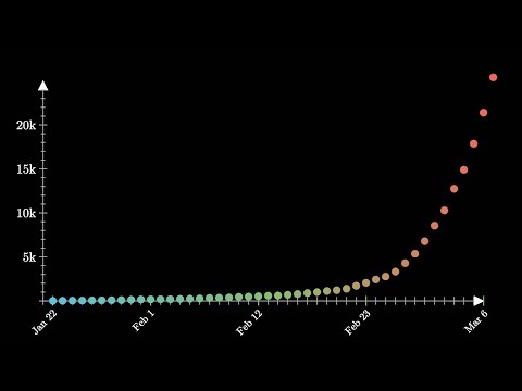
3Blue1Brown: Exponential growth and epidemics. Watch for how a constant growth factor makes a straight line on a logarithmic scale, and for the point where exponential growth must bend into a slower, logistic curve.

✦

Practice

Give answers to 3 significant figures unless told otherwise. Money figures are illustrative.

A culture of bacteria grows as $N = 500e^{0.4t}$ , with $t$ in hours. Find (a) $N$ after 5 hours (b) the doubling time (c) the rate of growth when $t = 5$ .
A quantity decays as $y = y_0 e^{-0.05t}$ . Find its half-life.
Use the NISR counts for 2002 (8 128 553) and 2012 (10 515 973) to find the continuous growth rate $k$ for that decade. Compare it with the 2012–2022 value, 0.0231.
How long does it take 200 000 Frw to grow to 300 000 Frw at 6% a year compounded continuously?
A loan of 2 000 000 Frw at 1.5% a month is repaid in 24 equal monthly payments. Find the monthly payment.
A bone has 60% of the carbon-14 of living bone. Estimate its age.
How many times more energy does a magnitude 7.0 earthquake release than a magnitude 5.0 earthquake?
A town's population was 40 000 in 2015 and 46 000 in 2020. Using an exponential model, in which year will it first exceed 60 000? Comment on the reliability of your answer.

Show answersHide answers

(a) $500e^{2} \approx 3690$ (b) $\frac{\ln 2}{0.4} \approx 1.73$ hours (c) $N' = 0.4N \approx 1480$ per hour.
$\frac{\ln 2}{0.05} \approx 13.9$ time units.
$k = \frac{1}{10}\ln\frac{10\,515\,973}{8\,128\,553} \approx 0.0258$ per year (2.6%), higher than 0.0231: growth slowed after 2012.
$e^{0.06t} = 1.5$ , $t = \frac{\ln 1.5}{0.06} \approx 6.76$ years.
$M = \frac{2\,000\,000 \times 0.015}{1 - 1.015^{-24}} \approx 99\,848$ Frw.
$t = -\frac{5730}{\ln 2}\ln 0.6 \approx 4220$ years.
$10^{1.5 \times 2} = 1000$ times.
$k = \frac{1}{5}\ln\frac{46\,000}{40\,000} \approx 0.0280$ . $40\,000e^{kt} = 60\,000$ gives $t = \frac{\ln 1.5}{k} \approx 14.5$ years after 2015, that is, during 2029. The model assumes the 2015–2020 rate lasts for another decade, so treat it as a rough estimate.

1Rwanda's population, 2012 to 2022

2Money: compound interest, loans and depreciation

3Decay: carbon-14 dating

4Earthquakes: a logarithmic scale

Rwanda's population, 2012 to 2022

Money: compound interest, loans and depreciation

Decay: carbon-14 dating

Earthquakes: a logarithmic scale